Central Limit Theorem: Why Averages Form a Bell Curve
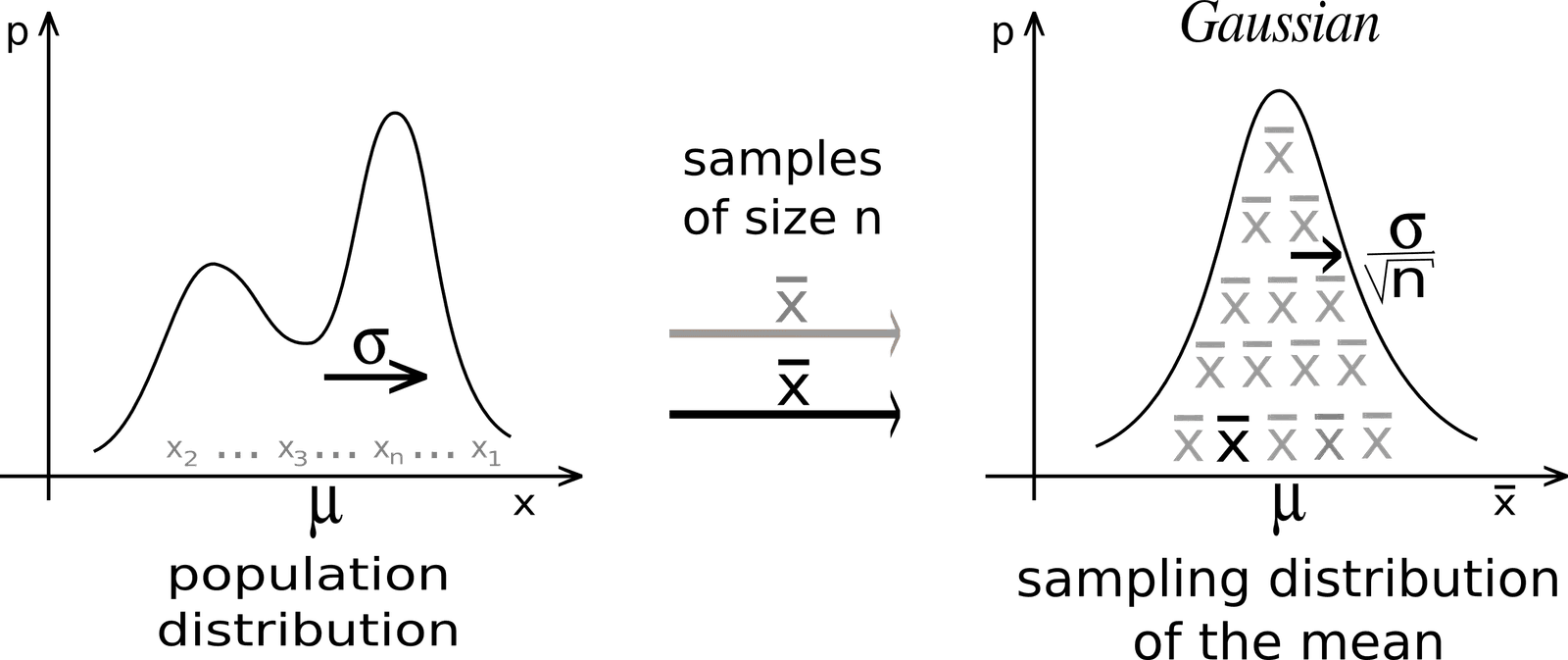
The Central Limit Theorem explains why averages of samples tend to form a bell curve, even if the original data doesn't. It's the foundation for A/B testing and quality control. The footgun is assuming it works for small or non-independent samples.
THE MENTAL MODEL: If you take many large enough samples from any population and calculate the mean of each sample, the collection of those means will be normally distributed (a bell curve). This is true even if the original population was, say, uniformly distributed like dice rolls. The theorem connects messy, real-world data to the predictable properties of the normal distribution, allowing us to make inferences with a known degree of confidence.
HOW IT WORKS: The power of the theorem comes from averaging. In any given sample, extreme high and low values tend to cancel each other out. When you plot the distribution of thousands of these sample means, they naturally cluster around the true population mean. A sample mean that is far from the true mean is statistically less likely to occur than one that is close. This tendency creates the characteristic bell shape. The resulting distribution of sample means will have a mean equal to the true population mean and a standard deviation that shrinks as your sample size grows.
WHEN TO USE IT: The CLT is the backbone of frequentist hypothesis testing. It's used whenever you need to infer properties of a large population from a smaller sample. Three key applications are: first, A/B testing, to determine if the average conversion rate of a new feature is statistically better than the old one; second, political polling, to estimate the true proportion of voters for a candidate from a sample of a few thousand people; and third, manufacturing quality control, to check if the average weight of a batch of products falls within an acceptable range.
WHEN NOT TO USE IT: The theorem is not a universal law and has important preconditions. Do not apply it when your samples are very small (a common but not rigid rule of thumb is a sample size below 30). It also fails if the samples are not independent; for example, sampling a stock price every second, where each price is highly correlated with the previous one. Finally, it does not apply to underlying distributions that lack a defined mean or variance, such as the Cauchy distribution, though these are rare in typical engineering problems.
ONE CANONICAL EXAMPLE: Imagine rolling a single fair six-sided die. The distribution of outcomes is uniform; each number from 1 to 6 has an equal 1/6 chance. Now, instead of one die, roll ten dice and calculate their average. Repeat this process thousands of times. If you plot a histogram of these thousands of averages, you will not see a flat, uniform line. You will see a distinct bell curve centered around 3.5, the true mean of a single die roll. The CLT perfectly predicts this transformation from a uniform to a normal distribution.
Read the original → en.wikipedia.org
Get five bites like this every day.
Tezvyn delivers a daily feed of 60-second tech bites with quizzes to lock in what you learn.